Objective 2.1#
LO# |
Description |
|---|---|
2.1 |
I can graph a given sinusoidal signal, including DC components, in both the time and frequency domains and determine its bandwidth. |
Motivation#
So far, we’ve only looked at very simple AC signals – sinusoids. However, real signals are inherenetly complex. Consider your favorite song - at any one point in time you will hear several instruments, which produce a range of frequencies. Can you imagine how difficult it would be to analyze the signal in the time domain? This is why, for highly complex signals, we typically analyze the signal with respect to frequency instead of time. Frequency domain representations allow us to view and manipulate signals in a more intuitive way. For example, if you wanted to add more bass and less treble to your song, you would use an equalizer. In essence, an equalizer is a simple filter – one that allows us to boost specific frequencies and reduce others. If you wanted more bass, then you could reduce the volume of the high frequencies while keeping the volume of the low frequencies the same. In this lesson, we will look at signals in the frequency domain.
Frequency Domain#
In Block I, we explained how the frequency of a sinusoid tells us the number of times the signal repeated (or “cycled”) in a second. To graph the signal as a function of time (or in the time domain), we translated the frequency into a period using the following equation:
When we start looking at moving information around, we will see that understanding how fast a signal changes is often more important than being able to trace it as it changes. Fast changing signals (with high frequencies) require us to collect more data to fully capture them.
The technique we will use to represent the frequency content of a message is known as an amplitude spectrum, or a plot or graph that describes a signal’s power or energy as a function of frequency. It is important to realize a signal does not exist exclusively in the time or frequency domain – those are simply different ways we choose to represent the signal. We can represent any signal as an equation, or as a combination of sines and cosines, which can then be viewed as a time domain waveform, or as an frequency spectrum plot. As we proceed further, it will become clearer there is a definite relationship between the two domains and each has its own usefulness. It is similar to looking at an object through regular binoculars or through night vision goggles – we see the same object, but it appears differently.
Let’s look at a sinusoid first. Electrical engineers like sinusoids because they are mathematically straightforward and very easy to analyze. In fact, in frequency domain there’s only one value on the x-axis instead of the infinite number of values for time we needed when we graphed sinusoids in time. So, for an amplitude spectrum, instead of plotting the function’s value on the y-axis and time on the x-axis, we will plot amplitude on the y-axis and frequency on the x-axis. To translate a signal from the time domain to the frequency domain, we only need to gather two pieces of information from the equation (or plot): amplitude and frequency. For example, if we wanted to graph the amplitude spectrum of the monotone signal:
we simply draw a vertical line at 440 Hz (the frequency of the cosine term), with an amplitude of 100mV, as shown below. What this means is that the signal, v(t), oscillates at a single frequency (400Hz) and we assume it never changes.
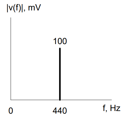
Figure 1: Frequency domain graph of a sinusoid with a frequency of 440 Hz
If we don’t worry about any phase shifts (and we won’t for the sake of this lesson), then we can say the graph above contains exactly the same information as the original equation. This is an important point. We now have three distinct and useful ways of representing an electrical signal:
An equation
A waveform (graphing voltage/current/power with respect to time)
An amplitude spectrum (graphing voltage/current/power with respect to frequency).
Now we can complicate things a little bit. True monotone (one single frequency) sinusoids don’t happen very often in the physical world. Even just a single note on an instrument contains to some additional tones, which are slightly above and below the primary frequency. Also, if we were to play the same note on a piano, it contains more than one harmonic (higher frequency). These harmonics give each instrument it’s unique sound. This is the reason why a piano sounds like a piano.
So, when we play an A above middle C on the piano, we get a signal with a fundamental frequency of 440 Hz, plus a series of harmonic frequencies, each one at a multiple of 440 Hz. Each successive harmonic exists at a lower amplitude than the one before it.
It is easy to imagine how graphing this signal in the time domain would become very complicated very quickly. But just to drive the point home, the figures on the next page show the first five harmonics of the 440Hz note in both the time domain (left) and frequency domain (right):
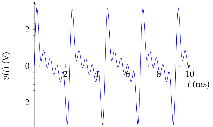
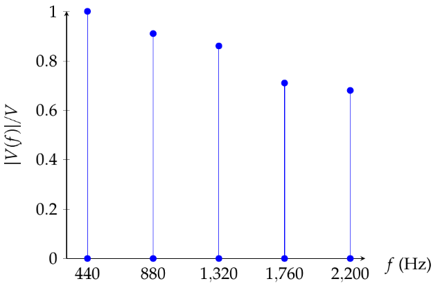
Figure 3: Frequency domain of first five harmonics of 440 Hz note
In theory, these harmonics continue out to infinity, each one located at a multiple of 440 Hz, but as we add more notes from more instruments, the signal becomes even more complex. If we really wanted, we could write the signal above as an equation:
Hopefully, you can see three things from this equation:
First, the time domain plot doesn’t give much useful information
Second, the equation is fairly tedious and not that easy to digest
Third, each vertical line in the graph corresponds to a single cosine term in the equation
DC Signals in the Frequency Domain#
DC signals in the frequency domain are important because sometimes we will want to add a bias to a signal. For example, let’s say that we want to add a DC bias of 50 mV to the 440Hz signal. The resulting formula for the voltage would be:
At first glance, this does not appear helpful, as the bias term has no cosine, and thus, no frequency. However, if we think of the DC voltage as not fluctuating with time, hence having a frequency of ‘zero’ hertz (0 Hz), and we keep in mind that the a cos(0) equals “1”, we could rewrite the above equation like this:
Now we see that we can simply draw a spike at ‘zero’ to represent the DC voltage.
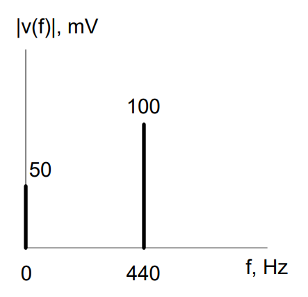
Figure 4: Frequency domain graph of signal with DC bias and 440 Hz sinusoid
Bandwidth#
Bandwidth is a very important term in ECE, and it refers to the range of frequencies that a signal or system contains. Many people like to use bandwidth to refer to cell phone or internet data rates, but for this class, we will keep these notions separate. A range of frequencies will be the bandwidth, and the speed at which you can transfer information on a computer or cell phone will be the data rate.
We can calculate the bandwidth of a signal or system by subtracting the lowest frequency from the highest frequency, as shown in the following equation.
For example, the bandwidth of the signal in Figure 4 is 440 Hz because \(f_{high} = 440\ Hz\) and \(f_{low} = 0\ Hz.\) For the signal in Figure 3, \(f_{high} = 2.2\ kHz\) and \(f_{low} = 440\ Hz\), so the bandwidth is 1.76 kHz. This brings us to two points. First, frequency domain graphs are very helpful for calculating the bandwidth of a signal. Second, the lowest frequency of a signal, \(f_{low}\), will only be 0 Hz if the signal has a DC bias.